Convolutions in Autoregressive Neural Networks

This post explains how to use one-dimensional causal and dilated convolutions in autoregressive neural networks such as WaveNet. For implementation details, I will use the notation of the tensorflow.keras.layers package, although the concepts themselves are framework-independent.

Say we have some temporal data, for example recordings of human speech. At a sample rate of 16,000 Hz, one second of recorded speech is a one-dimensional array of 16,000 values, as visualized here. Based on the recordings we have, we can compute a probabilistic model of the value at the next time step given the values at the previous time steps. Having a good model for this would be really helpful as it would allow us to generate speech ourselves.

A simple approach would be to model the next value using an affine transformation (linear combination + bias) of the four previous values. Implemented in Keras, this would be a single Dense layer with units=1:

This is already an autoregressive neural network. We can train it by splitting our recordings into appropriate chunks of inputs and targets, i.e.:

1st chunk: x = [1, 2, 3, 4], y = [5]
2nd chunk: x = [2, 3, 4, 5], y = [6]
3rd chunk: x = [3, 4, 5, 6], y = [7]
...

But since we only predict one time step per feed-forward pass, it takes long to iterate through a single training example, let alone through our entire dataset. It would speed up training if we could predict the next time steps for a whole training example in a single feed-forward pass. To do this, we need to apply the same four weights to each chunk of time steps in the input frame. This is exactly what a Conv1D layer with kernel_size=4 does:

So, training a fully connected layer in theory corresponds to training a convolutional layer in practice. Note that the final trained model is still a fully connected layer. We just train it efficiently by converting it to a convolutional layer without changing the number or shape of the weights.

At this point, we are already using causal convolutions. This might be surprising, because we just defined a simple convolutional layer without specifying something like causal=True. But whether a convolution is causal or not is rather a matter of perspective than of the architecture. By using it in a causal way, i.e. giving the model appropriate input and target values, we make it a causal convolution. We could also decide to use the same convolutional layer in a non-causal way, for example for processing an image. Then, our view of it would look like this:

This causal interpretation also works for a neural network with multiple layers. We only have to make sure that the time step given as the target value comes after the final layer's receptive field. Thus, the model never has access to future time steps when predicting the value of the next one.

Causal padding

One thing that Conv1D does allow us to specify is padding="causal". This simply pads the layer's input with zeros in the front so that we can also predict the values of early time steps in the frame:

This doesn't change the architecture of our model (it's still a fully connected layer with four weights). But it allows us to train the model on incomplete inputs. Thus, it also learns how to start a sequence (sentence, song etc.) and not just how to continue it. A convenient consequence of causal padding is that the output of a layer has the same width as its input. This is helpful when implementing skip connections between layers, which we will cover below.

Note: in the following, I will distinguish between the model's architecture "in theory" and the model's architecture "in practice". The former term refers to the concept of our model, which has been a single Dense layer with four weights so far. The latter term refers to the architecture we use for training the model efficiently. Above, we have seen that in order to train the model efficiently, we should use a Conv1D layer instead of a Dense layer. This, however, does not change the model's parameters. It is just a trick used for training. At test time, our model can be converted to a Dense layer again.

Convolutions in theory

Above, we have seen that a fully connected layer in theory corresponds to training a convolutional layer in practice. But what does a convolutional layer in theory correspond to? For example, this convolutional neural network:

The lower layer is a convolutional layer. The upper layer can be seen as a fully connected layer or as a convolutional layer with a feature map of size one. Now, when drawing the computations for the other time steps with dashed arrows, we see that we can use convolutional layers in practice as well:

Dilated convolutions

When a convolutional layer in our conceptual architecture has a stride that is larger than one, for example

the subsequent layers in practice must compensate for this by leaving out the corresponding weights:

This is precisely what a dilated convolution does. It is equivalent to a convolution with a stride of greater than one in the previous layers. At the same time, it allows us to perform the actual convolution with a stride of one. This is necessary, since we want to apply our model to every time step in one feed-forward pass without skipping time steps. When taking a look at the WaveNet architecture (source), we can see that it theoretically also corresponds to a simple stack of convolutions with stride two:

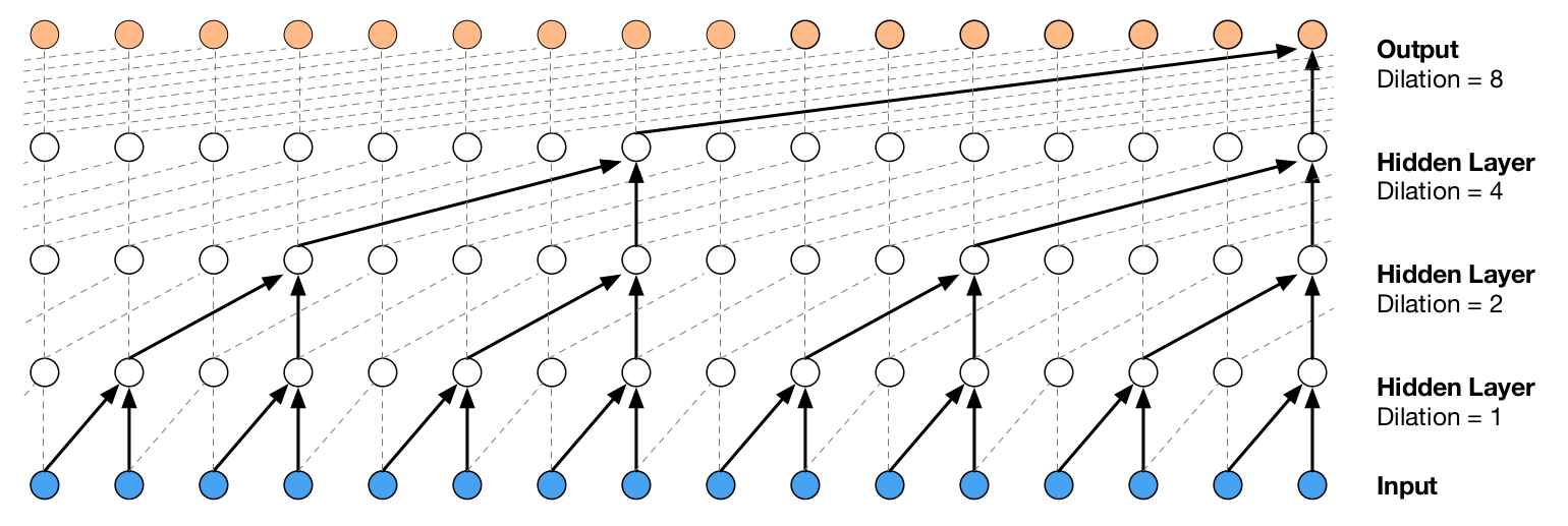
This figure shows how a stride greater than one affects the dilation rates of all subsequent layers in practice, not just the next one. For example, the dilation rate in the output layer is 2 * 2 * 2 = 8, caused by the "conceptual strides" in the previous layers. If we set the conceptual stride in the layer before the output layer to 1, the output layer would still need a dilation rate of 4. The rule for computing the dilation rate in a specific layer is to multiply all conceptual strides of the previous layers (more on the equivalence of strides and dilation rates below).

Pooling

Pooling is problematic when we perform it on the output of a convolutional layer with a stride larger than one. In theory, that would look like this:

When drawing the arrows for the computation of the previous time step, we can see that a problem arises in the neurons marked with exclamation marks.

These neurons don't appear in the conceptual computation of the tenth time step, yet they are included in the pooling windows and thus will influence the computation in practice. What we need to circumvent this is a pooling layer with dilation; just like in the convolutional layers. Unfortunately, the pooling layers AvgPool1D and MaxPool1D neither support dilation rates nor specifying padding="causal". We can, however, use tf.nn.pool, which supports specifying a dilation rate. As for the causal padding, we can take a look at Keras' implementation to verify that we can really just pad the input on the left and then carry on with "valid" padding:

if padding == 'causal':
    # causal (dilated) convolution:
    left_pad = dilation_rate * (kernel_shape[0] - 1)
    x = temporal_padding(x, (left_pad, 0))
    padding = 'valid'

Below is a custom Keras layer that will perform dilated pooling with optional causal padding. The pooling_type argument is given to tf.nn.pool and must be "avg" or "max" (case insensitive).

import tensorflow as tf

class DilatedPooling1D(tf.keras.layers.Layer):
    def __init__(self, pooling_type, pool_size=2, padding='causal',
                 dilation_rate=1, name=None, **kwargs):
        super(DilatedPooling1D, self).__init__(name=name, **kwargs)
        self.pooling_type = pooling_type.upper()
        self.pool_size = pool_size
        self.padding = padding.upper()
        self.dilation_rate = dilation_rate
        self.input_spec = tf.keras.layers.InputSpec(ndim=3)

    def call(self, inputs):
        # Input should have rank 3 and be in NWC format
        padding = self.padding
        if self.padding == 'CAUSAL':
            # Compute the causal padding
            left_pad = self.dilation_rate * (self.pool_size - 1)
            inputs = tf.pad(inputs, [[0, 0, ], [left_pad, 0], [0, 0]])
            padding = 'VALID'

        outputs = tf.nn.pool(inputs,
                             window_shape=[self.pool_size],
                             pooling_type=self.pooling_type,
                             padding=padding,
                             dilation_rate=[self.dilation_rate],
                             strides=[1],
                             data_format='NWC')
        return outputs

Fully connected layers

The fully connected layers above all had a single unit and could be interpreted as convolutional layers with a feature map of size one. Fully connected layers with multiple units can be interpreted as convolutional layers as well by setting the number of filters to the number of units while each feature map still has a size of one. For example, when adding a softmax output layer to our conceptual architecture, we add a convolutional layer with filters = n_classes.

Thus, we can directly draw the network architecture in practice:

This also works for hidden fully connected layers. Many convolutional neural networks have large fully connected layers before the softmax output layer, for example

model = Sequential([
    ..., # Output of this part has the shape (batch_size, 10, 32)
    Flatten(),
    Dense(units=500, activation='relu'),
    Dense(units=100, activation='relu'),
    Dense(units=10, activation='softmax'),
])

Regardless of whether the network is autoregressive or not, this is equivalent to

model = Sequential([
    ..., # Output of this part has the shape (batch_size, 10, 32)
    Conv1D(filters=500, kernel_size=10, padding='valid', activation='relu'),
    Conv1D(filters=100, kernel_size=1, padding='valid', activation='relu'),
    Conv1D(filters=10, kernel_size=1, padding='valid', activation='softmax'),
])

Therefore, we can use fully connected layers in our conceptual architecture just like convolutional layers.

Skip connections

Another popular architectural concept are residual and skip connections. The WaveNet architecture makes use of these as well. Since causal padding makes the outputs of all layers have the same width, residual connections are simple to implement in the network used for training:

Here, we add the blue input values to the output of the first hidden layer. We also add the result to the output of the second hidden layer. In the conceptual network, i.e. our final trained network, this corresponds to adding residual connections to the first time step in each convolution's receptive field:

An alternative to adding the skip connection to a layer's output, for example adding the blue input values to the output of the first hidden layer, is to simply concatenate the feature maps of both tensors. DenseNet uses this approach to give layers close to the output direct access to layers close to the input. An advantage of this method is that it does not require the same number of feature maps in each tensor. They need to match when using residual connections, because we add both tensors together, which might require using 1x1 convolutions. For concatenating them, however, they don't need to match. Each feature map just needs to have the same size, which they do when using causal padding.

When replacing the addition of the residual connections with a concatenation and adding a skip connection from the input to the second hidden layer, this is the resulting network architecture used during training:

The blue input values are now given as an input to the second hidden layer in a separate feature map. The feature maps of all three layer outputs are concatenated to be the input to whatever layer might follow after the second hidden layer. Just like with the residual connections, this corresponds conceptually to prioritizing more recent time steps - this time by assigning additional weights to them:

Mixing stride with dilation

The Conv1D layer does not support specifying both a stride greater than one and a dilation rate greater than one. One reason for this might be that you can express a network using strides and dilation rates greater than one with a network without strides greater than one. An example is the following (a bit crazy) network:

The boxes on the left show the original specification with strides greater than one while the boxes on the right show the corresponding specification with strides equal to one. While both specifications yield the same value in the output node, the specification on the right allows us to compute the outputs for multiple time steps in a single feed-forward pass. If we would use strides greater than one in the actual network used for training, we would skip time steps during that feed-forward pass.

"same" padding

One frequent architectural concept that cannot be easily translated into an efficient training architecture is "same" padding, at least I couldn't think of a solution for it. Conceptually, "same" padding looks like this:

We add padding on both sides of the input so that the size of each feature map in the layer's output is equal to the size of each input feature map (when using a stride of one). When applying this network to a whole frame of inputs in parallel, we notice that the space where the padding neurons need to be is occupied by the input values of other time steps - in this case the fourth input:

So, we can't apply our trick for efficient training to a conceptual model with "same" padding.

That's it, I hope you enjoyed this post! Let me know if you spot any errors or have an idea on how to make "same" padding work efficiently.

You can also leave a comment if you have a GitHub account. The "Sign in" button will store the GitHub API token in a cookie.