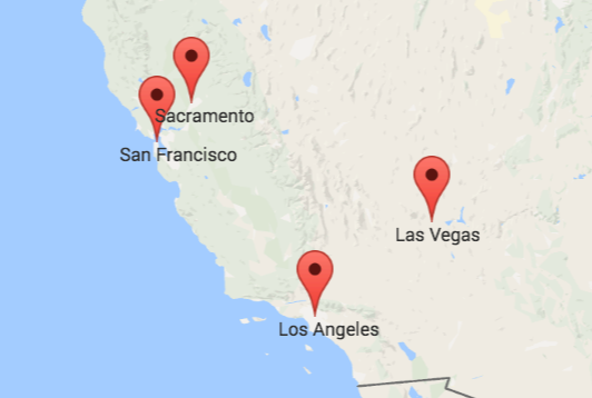
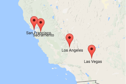
In a geography exam, the correct answer would be the left or upper one. It displays the actual locations of four cities in the US. But that does not make the other map entirely incorrect. It just displays other data. Specifically, it approximates the travel times between the four cities. This means that the closer two cities are on the right map the faster you can travel between them with public transport. We can calculate such maps using Multidimensional Scaling. What is Multidimensional Scaling? How can it help us to approximate travel times? And what is the relationship between the left map with the geographic locations and the right map? We are about to find out.
Task
Take a look at the following table.| From \ To | San Francisco | Sacramento | Los Angeles | Las Vegas |
|---|---|---|---|---|
| San Francisco | - | 121 km | 559 km | 671 km |
| Sacramento | 121 km | - | 582 km | 622 km |
| Los Angeles | 559 km | 582 km | - | 368 km |
| Las Vegas | 671 km | 622 km | 368 km | - |
| From \ To | San Francisco | Sacramento | Los Angeles | Las Vegas |
|---|---|---|---|---|
| San Francisco | - | 1 h 50 min | 7 h 18 min | 17 h 7 min |
| Sacramento | 2 h 12 min | - | 11 h 30 min | 16 h 51 min |
| Los Angeles | 7 h 40 min | 10 h 0 min | - | 6 h 14 min |
| Las Vegas | 14 h 45 min | 18 h 28 min | 6 h 5 min | - |
The similarity of both color maps shows that, generally, the travel time is proportional to the distance between two cities. However, there are small irregularities: the distance between San Francisco and Los Angeles is in the same ballpark as the distance between San Francisco and Las Vegas. Yet, the time needed to travel to Las Vegas is more than twice the time needed to travel to Los Angeles from San Francisco. So, either San Francisco and Los Angeles are connected exceptionally well or San Francisco and Las Vegas exceptionally badly.
Overall, we see that the distance between two cities does not necessarily correspond to their proximity by public transport. So, if we try to visualize how well cities are connected to each other, their actual geolocation may not be representative. A better solution is to take the table of travel times and calculate a list of coordinates so that the distances between those positions resemble the travel times as best as possible. I will describe the required steps in detail below. But first, you can take a look at the result:
Result
I created a small tool to visualize the results of this post. In the upper left corner of the map below, you will find a search box. Select three to ten cities which are reachable by public transportation. In the left or upper map, you will see their actual locations. The right or lower map will display the cities in a way that well-connected cities are closer to each other.Distances:
Travel durations by public transport (next Monday at 12 pm in the time zone of the first city):
Solution
Given: The cities' geographic locations and a matrix of travel times between their central stations.Multidimensional Scaling
We start with the matrix of travel times. Given a matrix of distances or dissimilarities between points, it is possible to calculate coordinates for each point that depict the similarities between the points when drawn onto a coordinate system. This is what Multidimensional Scaling (MDS) does. However, the distance between two points in the coordinate system may not always be equal to the value given by the matrix. Imagine a matrix with small entries for A-B and B-C but a very large entry for A-C. How can you draw A, B and C into a coordinate system without breaking the constraints given by the matrix?
Considering that a perfect solution might not exist, we therefore try to find points that approximate the given travel times best. This is similar to comparing the distances table with the travel durations table above, except now we may alter the cities' geographic coordinates to make both tables look as similar as possible. Specifically, we define "similar" via the squared difference between the distance between two points and the travel duration between the corresponding cities. Given a matrix \(A\), where \(a_{i,j}\) denotes the seconds needed to travel from city \(i\) to city \(j\), and the tuple \(P\) containing \(N\) two-dimensional points \(\{p_1, ..., p_N\}\), the overall error \(e(P)\) is defined as $$e(P) = \frac{1}{N^2}\sum _{i=1}^{N}{~} \sum _{j=1}^{N}{~}(a_{i,j}~-~dist(p_i,~p_j))^2$$ with \(dist(p_i, p_j)\) being the Euclidean distance between \(p_i\) and \(p_j\). For our purpose, it would be better to instead use the great-circle distance between points on a sphere. However, Multidimensional Scaling is not restricted to geographic applications, but can be used to visualize any matrix of dissimilarity values, including dissimilarities between breakfast cereals, legal offences and water samples from wells. Therefore, classical Multidimensional Scaling maps points into an abstract n-dimensional Euclidean space.
Classical Multidimensional Scaling
Update (21 June 2020) : Initially, I used Ben Frederickson's implementation of the classical MDS algorithm. I later discovered the following note in a derivation of this algorithm:
"When the observed proximity matrix is not Euclidean, the matrix B is not positive-definite. In such case, some of the eigenvalues of B will be negative; correspondingly, some coordinate values will be complex numbers. If B has only a small number of small negative eigenvalues, it's still possible to use the eigenvectors associated with the q largest positive eigenvalues"
(for details, please refer to these slides). While the algorithm produces reasonable approximations for every set of cities that I have entered so far, I wondered whether the condition mentioned in the last sentence of the quote was true in every case. After all, public transport can be pretty non-linear. Out of interest, I therefore implemented gradient descent for solving a Multidimensional Scaling problem and compared its solution to the one produced by the classical MDS algorithm.
The classical MDS algorithm assumes that the given distance matrix contains Euclidean distances. Using the Singular Value Decomposition of the centered squared distance matrix, it computes a tuple of points with optimal coordinates, minimizing the sum of squared errors above (the details of this can be found here). However, since trains do not always go the same speed and not every city is directly connected to all others, the algorithm's assumption does not apply in our case. While it still produces reasonable approximations, the results turn out to be suboptimal.
Iterative Optimization
Therefore, I tried out using gradient descent to see if it finds better solutions. There are better ways to perform Multidimensional Scaling (see "Modern Multidimensional Scaling - Theory and Applications" by Borg and Groenen for a comprehensive overview), but I was curious about how well gradient descent would perform.
Since the error function is quite simple, implementing its gradient was straightforward. I also tried out TensorFlow.js for differentiating the error function automatically, but found it to be orders of magnitude slower than computing the gradient directly (with 800 kilobytes, the library is also quite heavy). Nevertheless, it was helpful for ensuring that the gradient computation is correct. Out of interest, I also implemented the Gauss-Newton algorithm for Multidimensional Scaling to see how fast it finds a solution. You can find the code for both iterative optimization algorithms, each one applicable to general MDS problems, at the bottom of this post. Here is how they compare to the classical MDS algorithm on the set of cities that you entered above:
"Gradient Descent" refers to gradient descent with a learning rate of 1, "Momentum" refers to gradient descent with a learning rate of 0.5 and a momentum of 0.5 and "Gauss-Newton" refers to the Gauss-Newton algorithm with a learning rate (\(\alpha\)) of 0.1. The error of each algorithm's final solution is appended in parentheses. I experimented a bit with the learning rates, but generally you should not take the error curves too seriously. The key takeaway is that they all usually find better solutions than the classical MDS algorithm. Another benefit of the gradient-based approach is that we can easily modify the error function to, for example, use the great-circle distance instead of the Euclidean distance for \(dist(p_i, p_j)\).
Back To Earth
The points obtained by Multidimensional Scaling lie in some abstract Euclidean space and will not match the geographic locations of the cities. This is due to two facts:
- The travel times are given in seconds on public transport, while the distances between cities are measured in meters. As these are two completely different scales, the points' coordinates first have to be scaled to a geometrically meaningful coordinate system.
- Rotating, reflecting or moving the tuple of points does not change the distances between them. So, even if we scale the points to match the cities' scale, they may be upside down or at a completely different place on the earth. But since the tuple's inner distances do not change, it is still the optimal solution for approximating the matrix of travel times.
In short, we have to scale, rotate, reflect and move the tuple of points in order to get meaningful results. Luckily, Shinji Umeyama provides an algorithm that does exactly this in "Least-squares estimation of transformation parameters between two point patterns" (IEEE Transactions on Pattern Analysis & Machine Intelligence, 1991). For two tuples of n-dimensional points, the algorithm computes the rotation, translation and scale parameters to transform the points in one tuple such that the sum of squared Euclidean distances between corresponding points in the two tuples is minimized. I uploaded a JavaScript implementation of Umeyama's algorithm that optionally allows reflections here.
However, we run into the same problem as above: the points are two-dimensional and the algorithm minimizes Euclidean distances, but the cities lie on a sphere and we should therefore minimize great-circle distances. So, now we have three options:
- Perform gradient-based optimization directly on geographic coordinates using great-circle distances.
- Search for or think of extensions of Multidimensional Scaling and similarity transformations to geographic coordinates.
- Hope that public transport near the poles or across the 180° line of longitude will not increase drastically in the near future. Then, we simply treat the two coordinates of each point as latitude and longitude and accept that the similarity transformation algorithm will focus a bit too much on matching coordinates of cities close to the poles. We also accept to be mocked by every geodesist, although I think most of them already stopped reading when we performed MDS in Euclidean space without thinking about map projections.
After a bit of option 2, I chose option 3. The resulting points, based on the MDS solution of vanilla gradient descent, are depicted in the right or lower map above.
Code
I uploaded the code for performing Multidimensional Scaling with gradient descent or the Gauss-Newton algorithm to GitHub, as well as the implementation of Shinji Umeyama's similarity transformation algorithm:
The code in these repositories is documented a bit more, but you can also take a quick look at the implementation below. As mentioned above, I sanity checked the gradient computation using TensorFlow.js.
/**
 * Transform a tuple of source points to match a tuple of target points
 * following equation 40, 41 and 42 of umeyama_1991.
 *
 * This function expects two mlMatrix.Matrix instances of the same shape
 * (m, n), where n is the number of points and m is the number of dimensions.
 * This is the shape used by umeyama_1991. m and n can take any positive value.
 *
 * The returned matrix contains the transformed points.
 *
 * @param {!mlMatrix.Matrix} fromPoints - the source points {x_1, ..., x_n}.
 * @param {!mlMatrix.Matrix} toPoints - the target points {y_1, ..., y_n}.
 * @param {boolean} allowReflection - If true, the source points may be
 *   reflected to achieve a better mean squared error.
 * @returns {mlMatrix.Matrix}
 */
function getSimilarityTransformation(fromPoints,
                                     toPoints,
                                     allowReflection = false) {
    const dimensions = fromPoints.rows;
    const numPoints = fromPoints.columns;

    // 1. Compute the rotation.
    const covarianceMatrix = getSimilarityTransformationCovariance(
        fromPoints,
        toPoints);

    const {
        svd,
        mirrorIdentityForSolution
    } = getSimilarityTransformationSvdWithMirrorIdentities(
        covarianceMatrix,
        allowReflection);

    const rotation = svd.U
        .mmul(mlMatrix.Matrix.diag(mirrorIdentityForSolution))
        .mmul(svd.V.transpose());

    // 2. Compute the scale.
    // The variance will first be a 1-D array and then reduced to a scalar.
    const summator = (sum, elem) => {
        return sum + elem;
    };
    const fromVariance = fromPoints
        .variance('row', {unbiased: false})
        .reduce(summator);

    let trace = 0;
    for (let dimension = 0; dimension < dimensions; dimension++) {
        const mirrorEntry = mirrorIdentityForSolution[dimension];
        trace += svd.diagonal[dimension] * mirrorEntry;
    }
    const scale = trace / fromVariance;

    // 3. Compute the translation.
    const fromMean = mlMatrix.Matrix.columnVector(fromPoints.mean('row'));
    const toMean = mlMatrix.Matrix.columnVector(toPoints.mean('row'));
    const translation = mlMatrix.Matrix.sub(
        toMean,
        mlMatrix.Matrix.mul(rotation.mmul(fromMean), scale));

    // 4. Transform the points.
    const transformedPoints = mlMatrix.Matrix.add(
        mlMatrix.Matrix.mul(rotation.mmul(fromPoints), scale),
        translation.repeat({columns: numPoints}));

    return transformedPoints;
}

/**
 * Compute the mean squared error of a given solution, following equation 1
 * in umeyama_1991.
 *
 * This function expects two mlMatrix.Matrix instances of the same shape
 * (m, n), where n is the number of points and m is the number of dimensions.
 * This is the shape used by umeyama_1991.
 *
 * @param {!mlMatrix.Matrix} transformedPoints - the solution, for example
 *   returned by getSimilarityTransformation(...).
 * @param {!mlMatrix.Matrix} toPoints - the target points {y_1, ..., y_n}.
 * @returns {number}
 */
function getSimilarityTransformationError(transformedPoints, toPoints) {
    const numPoints = transformedPoints.columns;
    const difference = mlMatrix.Matrix.sub(toPoints, transformedPoints);
    return Math.pow(difference.norm('frobenius'), 2) / numPoints;
}

/**
 * Compute the minimum possible mean squared error for a given problem,
 * following equation 33 in umeyama_1991.
 *
 * This function expects two mlMatrix.Matrix instances of the same shape
 * (m, n), where n is the number of points and m is the number of dimensions.
 * This is the shape used by umeyama_1991. m and n can take any positive value.
 *
 * @param {!mlMatrix.Matrix} fromPoints - the source points {x_1, ..., x_n}.
 * @param {!mlMatrix.Matrix} toPoints - the target points {y_1, ..., y_n}.
 * @param {boolean} allowReflection - If true, the source points may be
 *   reflected to achieve a better mean squared error.
 * @returns {number}
 */
function getSimilarityTransformationErrorBound(fromPoints,
                                               toPoints,
                                               allowReflection = false) {
    const dimensions = fromPoints.rows;

    // The variances will first be 1-D arrays and then reduced to a scalar.
    const summator = (sum, elem) => {
        return sum + elem;
    };
    const fromVariance = fromPoints
        .variance('row', {unbiased: false})
        .reduce(summator);
    const toVariance = toPoints
        .variance('row', {unbiased: false})
        .reduce(summator);
    const covarianceMatrix = getSimilarityTransformationCovariance(
        fromPoints,
        toPoints);

    const {
        svd,
        mirrorIdentityForErrorBound
    } = getSimilarityTransformationSvdWithMirrorIdentities(
        covarianceMatrix,
        allowReflection);

    let trace = 0;
    for (let dimension = 0; dimension < dimensions; dimension++) {
        const mirrorEntry = mirrorIdentityForErrorBound[dimension];
        trace += svd.diagonal[dimension] * mirrorEntry;
    }
    return toVariance - Math.pow(trace, 2) / fromVariance;
}

/**
 * Computes the covariance matrix of the source points and the target points
 * following equation 38 in umeyama_1991.
 *
 * This function expects two mlMatrix.Matrix instances of the same shape
 * (m, n), where n is the number of points and m is the number of dimensions.
 * This is the shape used by umeyama_1991. m and n can take any positive value.
 *
 * @param {!mlMatrix.Matrix} fromPoints - the source points {x_1, ..., x_n}.
 * @param {!mlMatrix.Matrix} toPoints - the target points {y_1, ..., y_n}.
 * @returns {mlMatrix.Matrix}
 */
function getSimilarityTransformationCovariance(fromPoints, toPoints) {
    const dimensions = fromPoints.rows;
    const numPoints = fromPoints.columns;
    const fromMean = mlMatrix.Matrix.columnVector(fromPoints.mean('row'));
    const toMean = mlMatrix.Matrix.columnVector(toPoints.mean('row'));

    const covariance = mlMatrix.Matrix.zeros(dimensions, dimensions);

    for (let pointIndex = 0; pointIndex < numPoints; pointIndex++) {
        const fromPoint = fromPoints.getColumnVector(pointIndex);
        const toPoint = toPoints.getColumnVector(pointIndex);
        const outer = mlMatrix.Matrix.sub(toPoint, toMean)
            .mmul(mlMatrix.Matrix.sub(fromPoint, fromMean).transpose());

        covariance.addM(mlMatrix.Matrix.div(outer, numPoints));
    }

    return covariance;
}

/**
 * Computes the SVD of the covariance matrix and returns the mirror identities
 * (called S in umeyama_1991), following equation 39 and 43 in umeyama_1991.
 *
 * See getSimilarityTransformationCovariance(...) for more details on how to
 * compute the covariance matrix.
 *
 * @param {!mlMatrix.Matrix} covarianceMatrix - the matrix returned by
 *   getSimilarityTransformationCovariance(...)
 * @param {boolean} allowReflection - If true, the source points may be
 *   reflected to achieve a better mean squared error.
 * @returns {{
 *   svd: mlMatrix.SVD,
 *   mirrorIdentityForErrorBound: number[],
 *   mirrorIdentityForSolution: number[]
 * }}
 */
function getSimilarityTransformationSvdWithMirrorIdentities(covarianceMatrix,
                                                            allowReflection) {
    // Compute the SVD.
    const dimensions = covarianceMatrix.rows;
    const svd = new mlMatrix.SVD(covarianceMatrix);

    // Compute the mirror identities based on the equations in umeyama_1991.
    let mirrorIdentityForErrorBound = Array(svd.diagonal.length).fill(1);
    let mirrorIdentityForSolution = Array(svd.diagonal.length).fill(1);
    if (!allowReflection) {
        // Compute equation 39 in umeyama_1991.
        if (mlMatrix.determinant(covarianceMatrix) < 0) {
            const lastIndex = mirrorIdentityForErrorBound.length - 1;
            mirrorIdentityForErrorBound[lastIndex] = -1;
        }

        // Check the rank condition mentioned directly after equation 43.
        mirrorIdentityForSolution = mirrorIdentityForErrorBound;
        if (svd.rank === dimensions - 1) {
            // Compute equation 43 in umeyama_1991.
            mirrorIdentityForSolution = Array(svd.diagonal.length).fill(1);
            if (mlMatrix.determinant(svd.U) * mlMatrix.determinant(svd.V) < 0) {
                const lastIndex = mirrorIdentityForSolution.length - 1;
                mirrorIdentityForSolution[lastIndex] = -1;
            }
        }
    }

    return {
        svd: svd,
        mirrorIdentityForErrorBound: mirrorIdentityForErrorBound,
        mirrorIdentityForSolution: mirrorIdentityForSolution
    }
}
Notes
- Transit vs. Driving: By a small modification of the JavaScript code, you can also calculate the driving durations (set
TRAVEL_MODEtogoogle.maps.TravelMode.DRIVING). I tried it out and the resulting map differed only slightly from the real map. So, driving durations seem to generally scale proportionally to distances between cities. - Credits to Ben Frederickson for providing insights and the JavaScript code used for classical Multidimensional Scaling.
Like what you read?
I don't use Google Analytics or Disqus because they require cookies. I would still like to know which posts are popular, so if you liked this post you can let me know here on the right.
You can also leave a comment if you have a GitHub account. The "Sign in" button will store the GitHub API token in a cookie.